Predicting on Real world Sunspot Dataset

This blog is to demonstrate how to use tensorflow to predict probability of occurence of sunspot

You can use the .ipnyb notebook that is given with the repo by downloading and starting a kernel.

For local computer, use jupyter notebook
For cloud usage, checkout Google colab

import tensorflow as tf
print(tf.__version__)

2.2.0-rc3

import numpy as np
import matplotlib.pyplot as plt
def plot_series(time, series, format="-", start=0, end=None):
    plt.plot(time[start:end], series[start:end], format)
    plt.xlabel("Time")
    plt.ylabel("Value")
    plt.grid(True)

First, Downloading the data..

!wget --no-check-certificate \
    https://raw.githubusercontent.com/jbrownlee/Datasets/master/daily-min-temperatures.csv \
    -O daily-min-temperatures.csv

--2020-05-01 11:07:07--  https://raw.githubusercontent.com/jbrownlee/Datasets/master/daily-min-temperatures.csv
Resolving raw.githubusercontent.com (raw.githubusercontent.com)... 151.101.0.133, 151.101.64.133, 151.101.128.133, ...
Connecting to raw.githubusercontent.com (raw.githubusercontent.com)|151.101.0.133|:443... connected.
HTTP request sent, awaiting response... 200 OK
Length: 67921 (66K) [text/plain]
Saving to: ‘daily-min-temperatures.csv’

daily-min-temperatu 100%[===================>]  66.33K  --.-KB/s    in 0.008s  

2020-05-01 11:07:08 (7.69 MB/s) - ‘daily-min-temperatures.csv’ saved [67921/67921]

Now that we downloaded the sunspot data, let us understand the structure of the .csv file using pandas. This step is not really necessary.

import pandas as pd
data = pd.read_csv('daily-min-temperatures.csv')
data.head()

	Date	Temp
0	1981-01-01	20.7
1	1981-01-02	17.9
2	1981-01-03	18.8
3	1981-01-04	14.6
4	1981-01-05	15.8

We do not need the first row,that’s why we have next(reader). In the for loop we are appending the temp values only, as float. After that we plot to see the series.

import csv
time_step = []
temps = []

with open('daily-min-temperatures.csv') as csvfile:
  reader = csv.reader(csvfile, delimiter=',')
  next(reader)
  step=0
  for row in reader:
    temps.append(float(row[1]))
    time_step.append(step)
    step = step + 1

series = np.array(temps)
time = np.array(time_step)
plt.figure(figsize=(10, 6))
plot_series(time, series)

png

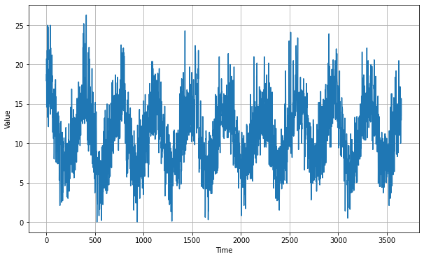
len(temps)

We are splitting the train and validation data as 2500 and 1150.

split_time = 2500
time_train = time[:split_time]
x_train = series[:split_time]
time_valid = time[split_time:]
x_valid = series[split_time:]

window_size = 30
batch_size = 32
shuffle_buffer_size = 1000

Below function windowed_dataset is used to create dataset usin tf.data.Dataset format. The model_forecast function is used to predict the values from the series provided. It also accepts the trained model as an arguement.

def windowed_dataset(series, window_size, batch_size, shuffle_buffer):
    series = tf.expand_dims(series, axis=-1)
    ds = tf.data.Dataset.from_tensor_slices(series)
    ds = ds.window(window_size + 1, shift=1, drop_remainder=True)
    ds = ds.flat_map(lambda w: w.batch(window_size + 1))
    ds = ds.shuffle(shuffle_buffer)
    ds = ds.map(lambda w: (w[:-1], w[1:]))
    return ds.batch(batch_size).prefetch(1)

def model_forecast(model, series, window_size):
    ds = tf.data.Dataset.from_tensor_slices(series)
    ds = ds.window(window_size, shift=1, drop_remainder=True)
    ds = ds.flat_map(lambda w: w.batch(window_size))
    ds = ds.batch(32).prefetch(1)
    forecast = model.predict(ds)
    return forecast

As we did in the previous blogs,after defining model structure, we are using tf.keras.callbacks.LearningRateScheduler to dynamically change the learning rate upon epochs. This will enable us to find the optimum learning rate.

Our model is a combination of Convolution and 2 LSTMs, both of which are bidirectional and having return_sequences as true. This improves the model mae but we have to check hoe accurate it will be after prediction and checking with validation set.

tf.keras.backend.clear_session()
tf.random.set_seed(51)
np.random.seed(51)
window_size = 64
batch_size = 256
train_set = windowed_dataset(x_train, window_size, batch_size, shuffle_buffer_size)
print(train_set)
print(x_train.shape)

model = tf.keras.models.Sequential([
  tf.keras.layers.Conv1D(filters=32, kernel_size=5,
                      strides=1, padding="causal",
                      activation="relu",
                      input_shape=[None, 1]),
  tf.keras.layers.LSTM(64, return_sequences=True),
  tf.keras.layers.LSTM(64, return_sequences=True),
  tf.keras.layers.Dense(30, activation="relu"),
  tf.keras.layers.Dense(10, activation="relu"),
  tf.keras.layers.Dense(1),
  tf.keras.layers.Lambda(lambda x: x * 400)
])

lr_schedule = tf.keras.callbacks.LearningRateScheduler(
    lambda epoch: 1e-8 * 10**(epoch / 20))
optimizer = tf.keras.optimizers.SGD(lr=1e-8, momentum=0.9)
model.compile(loss=tf.keras.losses.Huber(),
              optimizer=optimizer,
              metrics=["mae"])
history = model.fit(train_set, epochs=100, callbacks=[lr_schedule])

<PrefetchDataset shapes: ((None, None, 1), (None, None, 1)), types: (tf.float64, tf.float64)>
(2500,)
Epoch 1/100
10/10 [==============================] - 0s 31ms/step - loss: 31.1706 - mae: 31.6550 - lr: 1.0000e-08
Epoch 2/100
10/10 [==============================] - 0s 23ms/step - loss: 30.5228 - mae: 31.0756 - lr: 1.1220e-08
Epoch 3/100
10/10 [==============================] - 0s 23ms/step - loss: 29.6681 - mae: 30.1801 - lr: 1.2589e-08
Epoch 4/100
10/10 [==============================] - 0s 24ms/step - loss: 28.6311 - mae: 29.0586 - lr: 1.4125e-08
Epoch 5/100
10/10 [==============================] - 0s 24ms/step - loss: 27.1851 - mae: 27.6945 - lr: 1.5849e-08
Epoch 6/100
10/10 [==============================] - 0s 24ms/step - loss: 25.5238 - mae: 25.9986 - lr: 1.7783e-08
Epoch 7/100
10/10 [==============================] - 0s 24ms/step - loss: 23.2871 - mae: 23.8429 - lr: 1.9953e-08
Epoch 8/100
10/10 [==============================] - 0s 24ms/step - loss: 20.5082 - mae: 21.1108 - lr: 2.2387e-08
Epoch 9/100
10/10 [==============================] - 0s 25ms/step - loss: 17.1935 - mae: 17.8091 - lr: 2.5119e-08
Epoch 10/100
10/10 [==============================] - 0s 23ms/step - loss: 13.4642 - mae: 14.1371 - lr: 2.8184e-08
Epoch 11/100
10/10 [==============================] - 0s 25ms/step - loss: 10.0364 - mae: 10.6152 - lr: 3.1623e-08
Epoch 12/100
10/10 [==============================] - 0s 23ms/step - loss: 7.5764 - mae: 8.1025 - lr: 3.5481e-08
Epoch 13/100
10/10 [==============================] - 0s 24ms/step - loss: 6.2482 - mae: 6.7711 - lr: 3.9811e-08
Epoch 14/100
10/10 [==============================] - 0s 24ms/step - loss: 5.6777 - mae: 6.1856 - lr: 4.4668e-08
Epoch 90/100
10/10 [==============================] - 0s 26ms/step - loss: 26.0024 - mae: 25.3163 - lr: 2.8184e-04
Epoch 91/100
10/10 [==============================] - 0s 26ms/step - loss: 39.1242 - mae: 41.0090 - lr: 3.1623e-04
Epoch 92/100
10/10 [==============================] - 0s 24ms/step - loss: 29.0936 - mae: 29.5980 - lr: 3.5481e-04
Epoch 93/100
10/10 [==============================] - 0s 24ms/step - loss: 33.0701 - mae: 32.9219 - lr: 3.9811e-04
Epoch 94/100
10/10 [==============================] - 0s 26ms/step - loss: 36.9112 - mae: 37.8804 - lr: 4.4668e-04
Epoch 95/100
10/10 [==============================] - 0s 27ms/step - loss: 41.6311 - mae: 41.2765 - lr: 5.0119e-04
Epoch 96/100
10/10 [==============================] - 0s 25ms/step - loss: 46.5597 - mae: 47.5416 - lr: 5.6234e-04
Epoch 97/100
10/10 [==============================] - 0s 24ms/step - loss: 52.5361 - mae: 52.1260 - lr: 6.3096e-04
Epoch 98/100
10/10 [==============================] - 0s 25ms/step - loss: 58.8236 - mae: 59.7652 - lr: 7.0795e-04
Epoch 99/100
10/10 [==============================] - 0s 25ms/step - loss: 66.3937 - mae: 65.8950 - lr: 7.9433e-04
Epoch 100/100
10/10 [==============================] - 0s 26ms/step - loss: 74.3771 - mae: 75.2363 - lr: 8.9125e-04

plt.semilogx(history.history["lr"], history.history["loss"])
plt.axis([1e-8, 1e-4, 0, 60])

(1e-08, 0.0001, 0.0, 60.0)

png

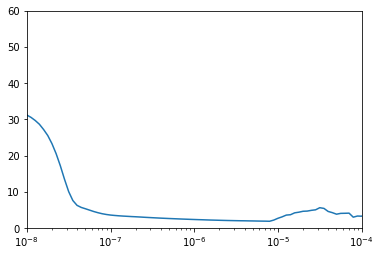
After plotting the graph we see that the loss is really low and stable for the learning_rate = $10^{-5}$. Now,we train using that learning rate.

tf.keras.backend.clear_session()
tf.random.set_seed(51)
np.random.seed(51)
train_set = windowed_dataset(x_train, window_size=60, batch_size=100, shuffle_buffer=shuffle_buffer_size)
model = tf.keras.models.Sequential([
  tf.keras.layers.Conv1D(filters=60, kernel_size=5,
                      strides=1, padding="causal",
                      activation="relu",
                      input_shape=[None, 1]),
  tf.keras.layers.LSTM(60, return_sequences=True),
  tf.keras.layers.LSTM(60, return_sequences=True),
  tf.keras.layers.Dense(30, activation="relu"),
  tf.keras.layers.Dense(10, activation="relu"),
  tf.keras.layers.Dense(1),
  tf.keras.layers.Lambda(lambda x: x * 400)
])


optimizer = tf.keras.optimizers.SGD(lr=1e-5, momentum=0.9)
model.compile(loss=tf.keras.losses.Huber(),
              optimizer=optimizer,
              metrics=["mae"])
history = model.fit(train_set,epochs=150)

Epoch 1/150
25/25 [==============================] - 0s 14ms/step - loss: 9.8211 - mae: 10.4694
Epoch 2/150
25/25 [==============================] - 0s 13ms/step - loss: 2.5191 - mae: 2.9923
Epoch 3/150
25/25 [==============================] - 0s 13ms/step - loss: 1.9513 - mae: 2.4047
Epoch 4/150
25/25 [==============================] - 0s 13ms/step - loss: 1.8610 - mae: 2.3151
Epoch 5/150
25/25 [==============================] - 0s 13ms/step - loss: 1.8209 - mae: 2.2733
Epoch 6/150
25/25 [==============================] - 0s 13ms/step - loss: 1.7905 - mae: 2.2418
Epoch 7/150
25/25 [==============================] - 0s 14ms/step - loss: 1.7667 - mae: 2.2186
Epoch 8/150
25/25 [==============================] - 0s 13ms/step - loss: 1.7387 - mae: 2.1906
Epoch 9/150
25/25 [==============================] - 0s 13ms/step - loss: 1.7173 - mae: 2.1681
Epoch 10/150
25/25 [==============================] - 0s 13ms/step - loss: 1.6987 - mae: 2.1482
Epoch 11/150
25/25 [==============================] - 0s 13ms/step - loss: 1.6815 - mae: 2.1287
Epoch 12/150
25/25 [==============================] - 0s 14ms/step - loss: 1.6685 - mae: 2.1159
Epoch 13/150
25/25 [==============================] - 0s 14ms/step - loss: 1.6576 - mae: 2.1030
Epoch 14/150
25/25 [==============================] - 0s 14ms/step - loss: 1.6430 - mae: 2.0891
Epoch 136/150
25/25 [==============================] - 0s 13ms/step - loss: 1.4917 - mae: 1.9333
Epoch 137/150
25/25 [==============================] - 0s 13ms/step - loss: 1.4946 - mae: 1.9363
Epoch 138/150
25/25 [==============================] - 0s 13ms/step - loss: 1.4904 - mae: 1.9329
Epoch 139/150
25/25 [==============================] - 0s 13ms/step - loss: 1.4885 - mae: 1.9321
Epoch 140/150
25/25 [==============================] - 0s 13ms/step - loss: 1.4897 - mae: 1.9325
Epoch 141/150
25/25 [==============================] - 0s 13ms/step - loss: 1.4902 - mae: 1.9311
Epoch 142/150
25/25 [==============================] - 0s 13ms/step - loss: 1.4900 - mae: 1.9304
Epoch 143/150
25/25 [==============================] - 0s 13ms/step - loss: 1.4916 - mae: 1.9333
Epoch 144/150
25/25 [==============================] - 0s 14ms/step - loss: 1.4909 - mae: 1.9326
Epoch 145/150
25/25 [==============================] - 0s 13ms/step - loss: 1.4887 - mae: 1.9299
Epoch 146/150
25/25 [==============================] - 0s 13ms/step - loss: 1.4943 - mae: 1.9364
Epoch 147/150
25/25 [==============================] - 0s 13ms/step - loss: 1.4889 - mae: 1.9306
Epoch 148/150
25/25 [==============================] - 0s 14ms/step - loss: 1.4882 - mae: 1.9300
Epoch 149/150
25/25 [==============================] - 0s 16ms/step - loss: 1.4900 - mae: 1.9307
Epoch 150/150
25/25 [==============================] - 0s 13ms/step - loss: 1.4886 - mae: 1.9292

rnn_forecast = model_forecast(model, series[..., np.newaxis], window_size)
rnn_forecast = rnn_forecast[split_time - window_size:-1, -1, 0]

We are removing the series data at time before split_time - window_size and then taking the data all the way to the end. After that, we plot to see the validation vs prediction.

plt.figure(figsize=(10, 6))
plot_series(time_valid, x_valid)
plot_series(time_valid, rnn_forecast)

png

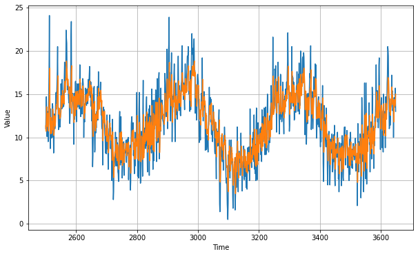
tf.keras.metrics.mean_absolute_error(x_valid, rnn_forecast).numpy()

1.7796258

The mean absolute error is really low compared to the other models we have tried out before. The next statement simply prints the forecasted values.

print(rnn_forecast)

[11.329356 10.705612 12.124963 ... 13.604561 13.796917 15.009445]

Tensorflow Sequence examples

Trying out Sequence model Prediction as part of Coursera tutorial

Predicting on Real world Sunspot Dataset